Exploratory Data Analysis

We wanted to build some intuition through EDA as to which features can provide good prediction. We will show some plots to understand the importance of features such as Game Location (Home vs Away vs Neutral), Momentum or Form factor (games won on a spree in the last N games), Team Chemistry (a higher standard deviation in players’ strength in a team indicates a low Team chemistry) and Team Strength based on Attack, Defense, Mid-field strengths of the players in a team.

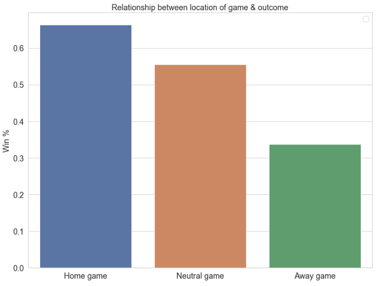
1. Game Location: We created a variable to indicate whether the game was played in Team 1’s country /continent or Team 2’s country/continent or at a neutral location. Although this is a simple feature, we plan to explore it a bit to see if “Home” advantage is crucial or not when other things are close enough. This is a common phenomenon in other sports where “conditions” make it favorable to the home team.

The summary graphic above shows that teams have a higher chance of winning when they are playing at home as compared to in neutral territory or even away (not considering Draw above). The feature we have created which indicates the game location seems to have relevancy for generating predictions of game outcomes. We will include country and continent as one of the predictors as it has the predictive power on the game outcome.

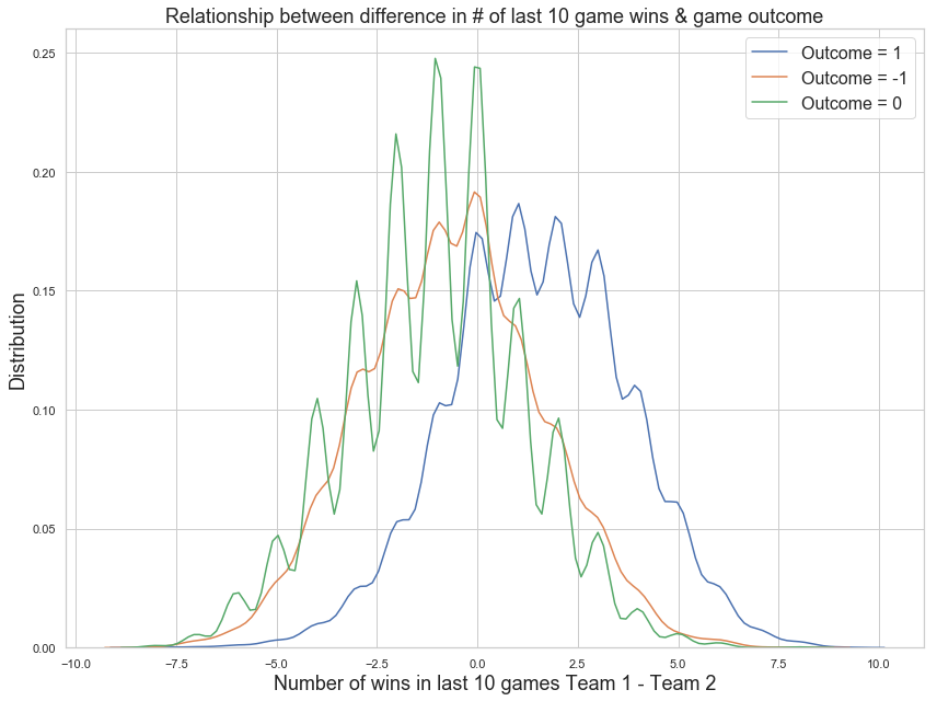
2. Form factor: We have created an additional feature that calculates the number of wins within the last 10 games for each team and each moment in time. This will serve as one proxy for the current form of a team. The original intuition here is that even if a team is historically a weak team its recent form weighs more and could give the teams performance a boost in moral and victory likelihood. Taking the difference between this metric for Team1 vs Team2 gives us a feature that emphasizes the relative difference in current form for each game. As can be seen here,  the difference in number of wins seems to have predictive power for determining if Team 1 wins (Outcome = 1) or Team 1 loses (Outcome = 0).  We will include form factor as one of the predictors as it seems to have the predictive power on the game outcome.

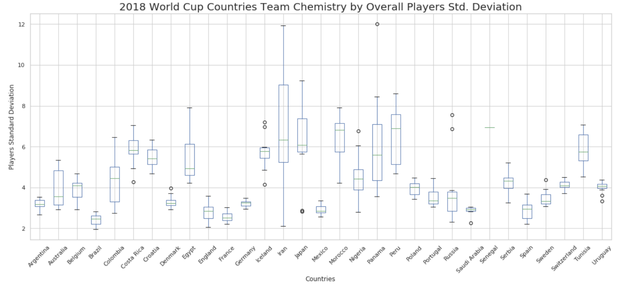
3.Team Chemistry: We know that one extraordinary player cannot do wonders in a team sport if there are many other players are very mediocre. Likewise, a team with many above average players could be a better team as they tend to have a better “coordination” or “chemistry”. To that point, we created a feature that is equal to the standard deviation of the players’ strengths within a team.  There were several limitations. First, “team chemistry” is a concept that might be very difficult to capture with numbers alone. There are factors such as emotions and bonding among players that cannot be easily captured by player strengths. This was just an attempt to capture part of the team chemistry and see if it helps in predicting better. There was a lot of effort that went into collecting and massaging the data. The problem was that the player strength data is available only for certain number of years in the past (2007 to 2017). Another issue was that it was available for players of only a smaller set of countries than the countries we have in our master game list. We made an attempt to reduce the master data for these countries and run models but they did not provide any better results. It was understandable because the team chemistry was a very crude estimate based on standard deviation of the player’s strength in a team, with an approximation that all those players were playing in that year. Although we did not include this feature in the final models in this project, we are interested to refine this in future but not in the scope of this project. Here is a box plot graph that shows all the World Cup qualifying countries team Chemistry over the years.

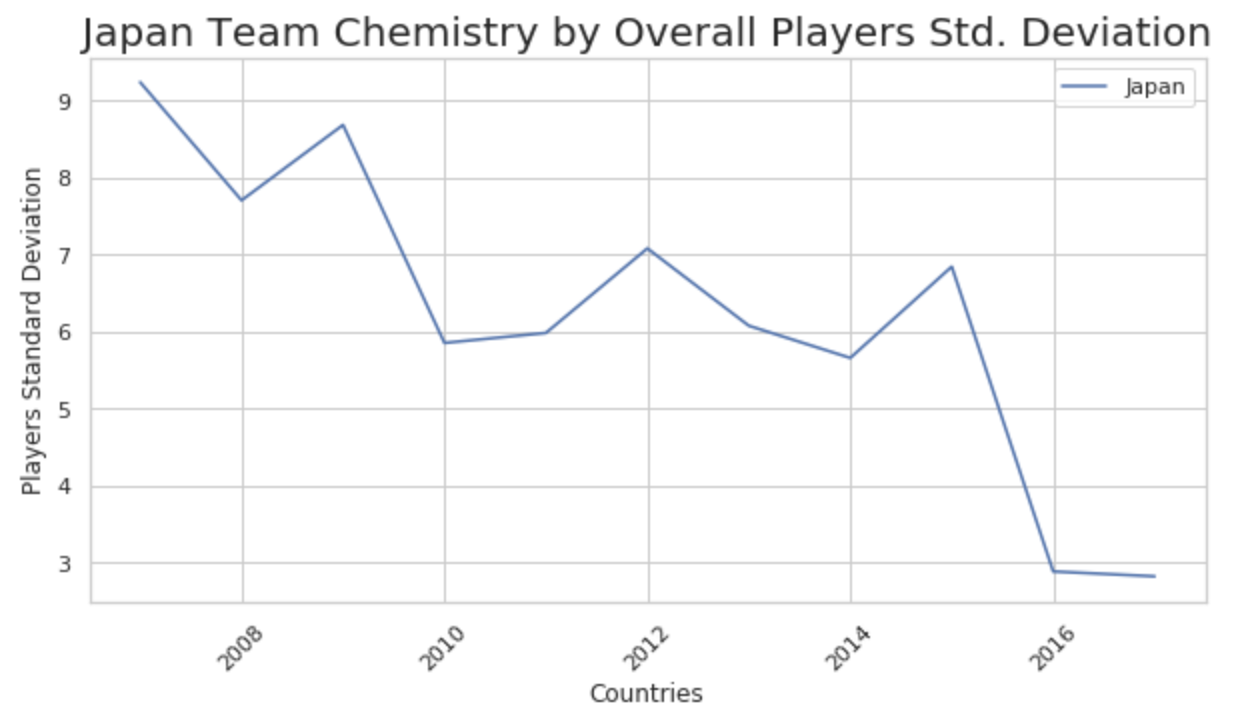
From the overall analysis we can see that the usual top teams have lower lower standard deviation of their players, teams like Brazil, France, Mexico, etc.  This shows that these teams consistently have strong chemistry through the years.  In some other case we see huge gap between the standard deviation of players this could indicates that either the team chemistry has improved or worsen over the years.  In order to dive a bit deeper into this relationship and see if there is a correlation between team chemistry and win ratio.  The below graphs will give a better view at one of the countries.

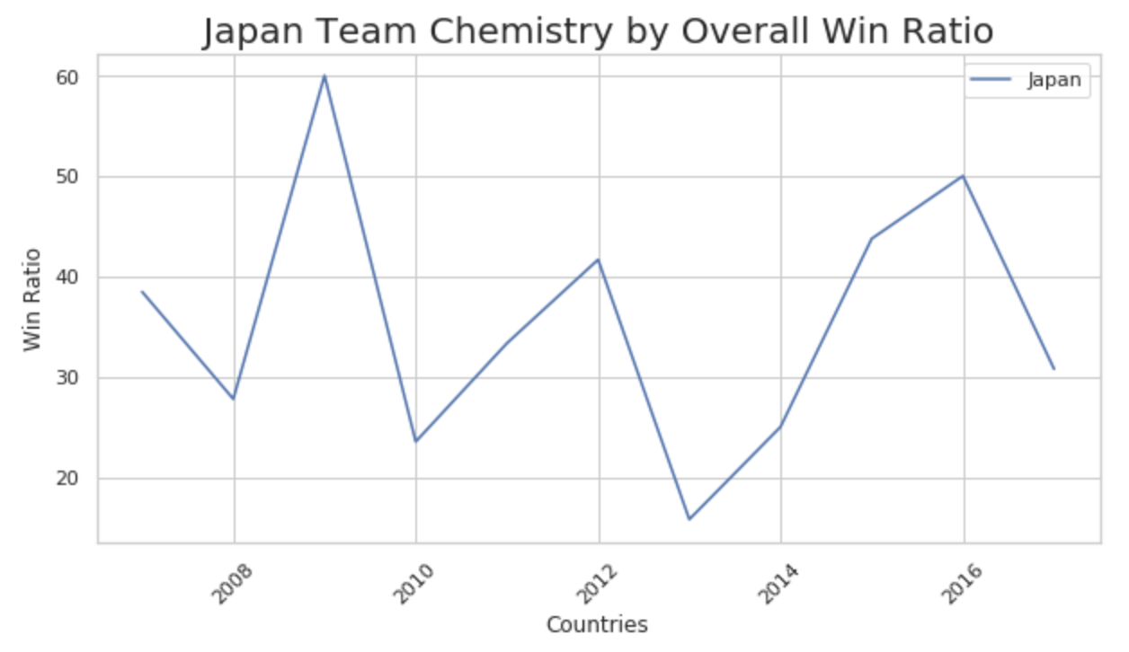
Unfortunately when we look at most of the countries like Japan there was a big correlation between the team chemistry and the win ratio.  If we look at year 2016 which shows a low standard deviation which should indicate excellent team chemistry, but when compared to the win ratio(win/loss) for the same year we can see that Japan won most of their games.  This is the correlation we wanted to see but instead when we compared year over year we can see that it did not show a nice correlation overall with the wins achieved in those years.

4. Team Strengths: Based on the players’ strength in Attack, Defense and Midfield, we wanted  to segregate the  strength of the team into three areas. In Soccer, we know that one team’s attack deals with the other team’s defense. So, it makes sense to use two scores by taking the difference between one team’s aggregate attack score and the other team’s aggregate defence score. They would probably be better indicators rather than considering differences of the same type (Team 1 Attack Score - Team 2 Attack score, for example). However, for midfield, it might make sense to consider the difference directly.

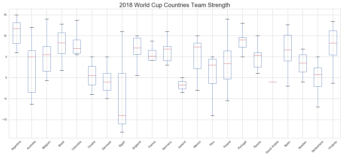
First, we will show raw team strength for 2018 World cup countries as a box plot to see how they differ.

The box-plot of team strength for 2018 world cup countries shows the median and spread of the team strength.  When we compare the median team strength score against the FIFA ranking, we found that the countries like Argentina and Belgium that have high team strength also have high FIFA rankings score (FIFA ranking: Argentina – 12, Belgium -1).  The countries like Egypt and Iceland that have low team strength also have low FIFA ranking score (FIFA ranking: Egypt – 58, and Iceland -36).  This shows some evidence that team strength would play a role in predicting the game outcome.  We will include team strength as one of the predictors in our model.

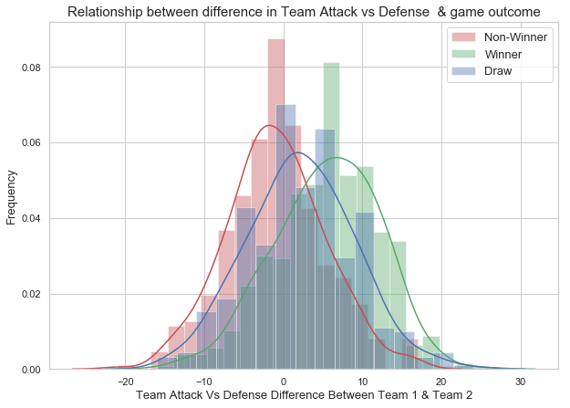
Team Attack vs Defense Difference

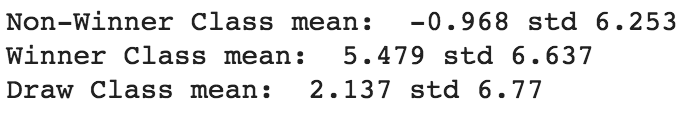
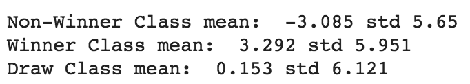
The attack vs defense-difference distribution plot shows that Winner and Non-winner classes are centered at different mean.  There is no significant difference in the standard deviation of the two distributions.  The mean attack difference of the winner class is +ve and non-winner class is -ve.  The +ve mean of the winner class indicates that the Winning team has higher attack vs defense score than the non-winning team. We also have the Draw class in the middle that is centered between the other two groups. The plot shows some evidence that the teams with more attack vs defense score will have more chances for winning.  We will include team attack vs defense difference as one of the predictor as it has the predictive power on the game outcome.

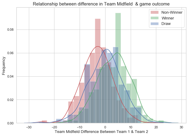
Midfield

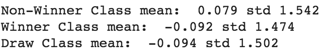
The midfield-difference plot shows that Winner and Non-winner classes are centered at different mean. The standard deviation of the winner class is slightly higher than the non-winner class.  The mean midfield difference of the winner class is +ve and non-winner class is -ve.  The +ve mean of the winner class indicates that the Winning team has higher midfield score than the non-winning team.  The plot shows some evidence that the teams with more midfield score will have more chances for winning.  We will include team midfield as one of the predictor as it has the predictive power on the game outcome.

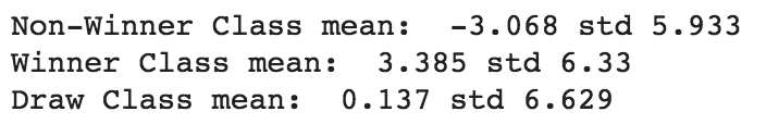
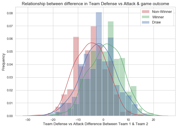
Team Defense Vs Attack Difference

The defense vs attack -difference plot shows that Winner and Non-winner classes are centered at different mean. The standard deviation of the winner class is slightly higher than the non-winner class.  The mean defense vs attack difference of the winner class is +ve and non-winner class is -ve.  The +ve mean of the winner class indicates that the Winning team has higher defense vs attack score than the non-winning team.  We also have the Draw class in the middle that is centered between those two other groups. The plot shows some evidence that the teams with more defense vs attack score will have more chances for winning.  We will include team defense vs attack as one of the predictor as it has the predictive power on the game outcome.

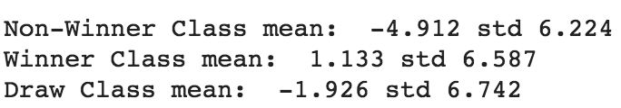
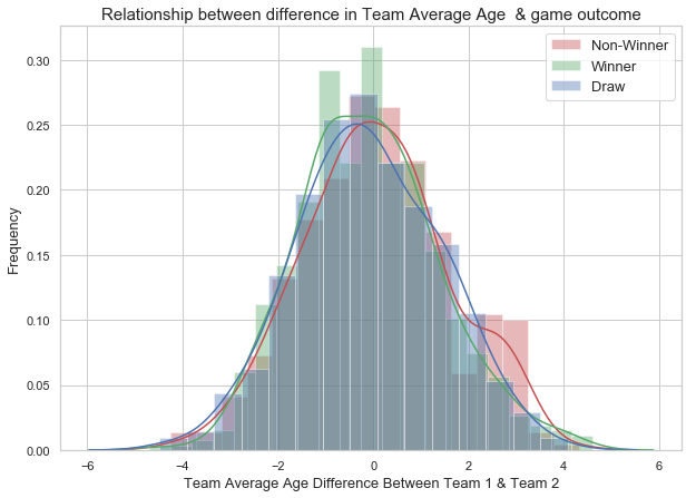
5. Average Age

The average-age-difference plot shows that Winner and Non-winner classes are centered at same mean, and have same standard deviation.  The plot clearly indicates that the average age does not differentiate winning team and non-winning team. Inclusion of Draw class also shows the same overlapping region and means.  We will not include average age as one of the predictor as it has the no predictive power on the game outcome.

6. Overall Team Strength

The overall-score-difference plot shows that Winner and Non-winner classes are centered at different mean. There is no significant difference in the standard deviation of both the classes.  The mean overall-score-difference of the winner class is +ve and non-winner class is -ve.  The +ve mean of the winner class indicates that the Winning team has higher overall score than the non-winning team.  We also have the Draw class in the middle that is centered around the zero. The plot shows some evidence that the teams with more defense score will have more chances for winning.  We will include team defense as one of the predictor as it has the predictive power on the game outcome.

7. Ranking difference

FIFA rankings is one of the important indicator of a team performance.  We would like to analyze the predictive power of the FIFA ranking. We have considered the difference between the ranking of teams in a game as a feature.  

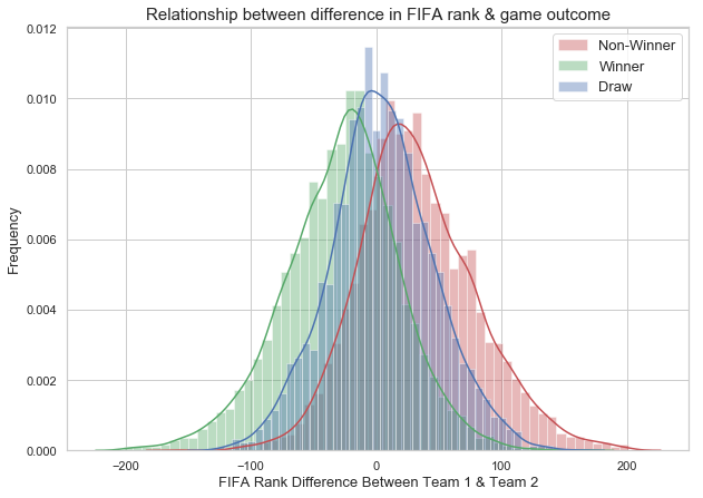
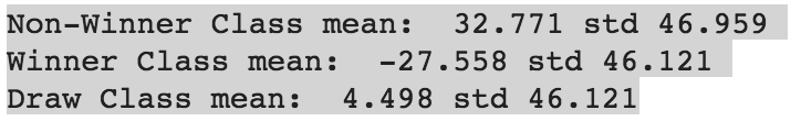
The FIFA-rank-difference plot shows that winner and non-winner classes are centered at different means.  There is no significant difference in the standard deviation of the two distributions.  The mean of the winner class is negative.  The negative rank-difference indicates that if teams with a better ranking will have lower FIFA rank value and therefore a lower score has an improved chance of winning the game. The lower the FIFA rank value, higher the overall performance. We also have the Draw class in the middle that is centered around the zero (similar rankings).  The plot shows some evidence that the teams with good FIFA rank will have more chances for winning.  We will include FIFA-rank-difference as one of the predictor as it has the predictive power of the game outcome.

Baseline Models

In our baseline models, we have considered three-category classification for the outcome.  The classes in the response variable are 1: Team-1 is a winner; 0: Draw and -1: Team-1 is a loser.

Random Generator:

The predicted outcome of the model is generated randomly which gives equal probability for Winner, Non-Winner and Draw classes.  

Input Data: Number of observations: 14256 (games conducted from 1993 to 2018)

Response Variable: Outcome (3-classes).

Result: Model Accuracy 0.336

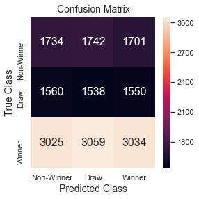
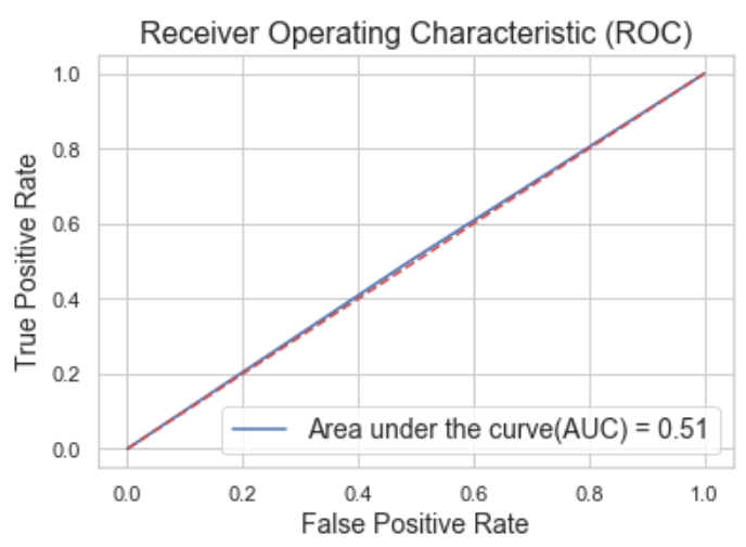
Confusion matrix and classification report shows that model has 33/33/33 chances of predicting Winner, Non-Winner and Draw classes.  ROC curve indicates the tradeoff between true positive rate (sensitivity) and false positive rate (1-specificity). Area under the curve is 0.51 which shows that the model is pure random on prediction.

Logistic Regression: 

We have built a logistic regression model as another baseline model with predictors: Game Location, Game Continent, Rank-difference, Team-1, Team-2; and Response Variable: Outcome (indicates if Team-1 is a Winner or Non-Winner).  The variables Team-1, Team-2, Game Location, and Game Continent are categorical variables and Rank-difference is a quantitative variable (Note: We tried another feature Stakes, which indicates the importance /seriousness of the game. However, looking at the model results, it was not a significant feature and had to be discarded).  Dummy variables are created for the categorical variables (for n categories, there are n-1 number of categorical variables).  We kept games from 1993 to 2017 for training, and 2018 games for testing.   Although in the final model we will be using just the games played during the FIFA world cup 2018 as test data, here, in the initial baseline model we have decided to utilize all 2018 games as a test data set.

Input Data: total records: 14256, # predictors: 7, response variable: 3-Outcomes

Training: number of records 14049 (1993 to 2017 games), predictors: 371 (after creating the categorical variables).  

Test: 2018 games

Model Result:  Accuracy on train=58.88%, test=54.46%

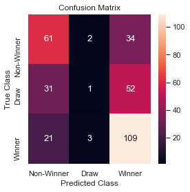
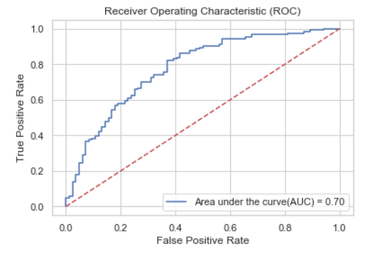
Confusion Matrix and ROC curve for test data.

The model results on test data show that the logistic regression model is more accurate than the random generate to predict the outcome of the game.  We also quickly checked the accuracy of the simple FIFA ranking model (58% on Training and 54% on the Test) and logistic regression model was doing reasonably better than the pure FIFA rank based prediction.