Feature Engineering and Final Models

Feature Engineering

Model Variables:

The variable outcome is set as the target variable.  The exploratory data analysis showed that form factor, FIFA ranks, Location of the game (country, continent), attack vs defense, dense vs attack, midfield and overall score have predictive power on the outcome of the game, we decided to include those in our model.  Though the distribution of the average age among three outcome groups (win, draw, & lose) does not show any significant difference, we decided to include variable team average age with the assumption that average age might have some interaction effect with other predictors.  In addition, we have included average population, distance between the team’s country.  We have spent lot of effort on collecting team chemistry data, but we could find the team chemistry record only for 230 observations in our model data, so we decided to drop that variable from the model.

Dummy Variables: Dummy variables are created for the categorical features, and the original categorical features are dropped from the input data matrix. while creating a set of dummy variables for a categorical feature with n categories, we dropped one category and created n-1 dummy variables.

Missing Values:  The features related to team strength have values only from 2007.  We wanted to experiment the models with different options for handling missing values.  

1. Drop records with missing values:  The observations with missing values will be removed from the input data matrix.
2. Drop Features with missing values:  The features related to team strength have no data prior to 2007 and will be removed from the input data matrix
3. Impute missing values:  Random Forest algorithm is used to impute the missing values.  Features with missing values are considered as target variables. The random forest model is trained on the data set with no missing values, and the trained model is used to predict the target variables with the missing values.  

Feature Scaling: StandardScaler is used to transform the all features with mean zero and standard deviation of 1.

Polynomial Features: we wanted to experiment our model with adding more polynomial features and interaction terms.

1. Power term: The polynomial features with degree 2 and 3 are created for the quantitative features: Rank_diff,RollingFormDiff,distance_diff, pop_diff,diffence_diff, attack_diff,

midfield_diff,age_diff,overall_diff.

2. Interaction terms: Interactions terms are creating by multiplying a set of categorical features with a set of quantitative features.

Interaction term 1 = [game_location_home, game_location_neutral]

Interaction term 2 = [Rank_diff, RollingFormDiff, diffence_diff, attack_diff, midfield_diff,  

                                     overall_diff]

Design Matrix:

Split x and y:

The variable Outcome is dropped from the input data matrix and considered as a target variable.  

Split Train and Test:

The world cup 2018 matches are dropped from the input data matrix and considering as test data set.  The remaining data are considered for model training the validation.  

Split train and Validation: 

20% of the random samples from the training data is removed for model cross validation and the remaining 80% of the data is used for model training.

Classification Models

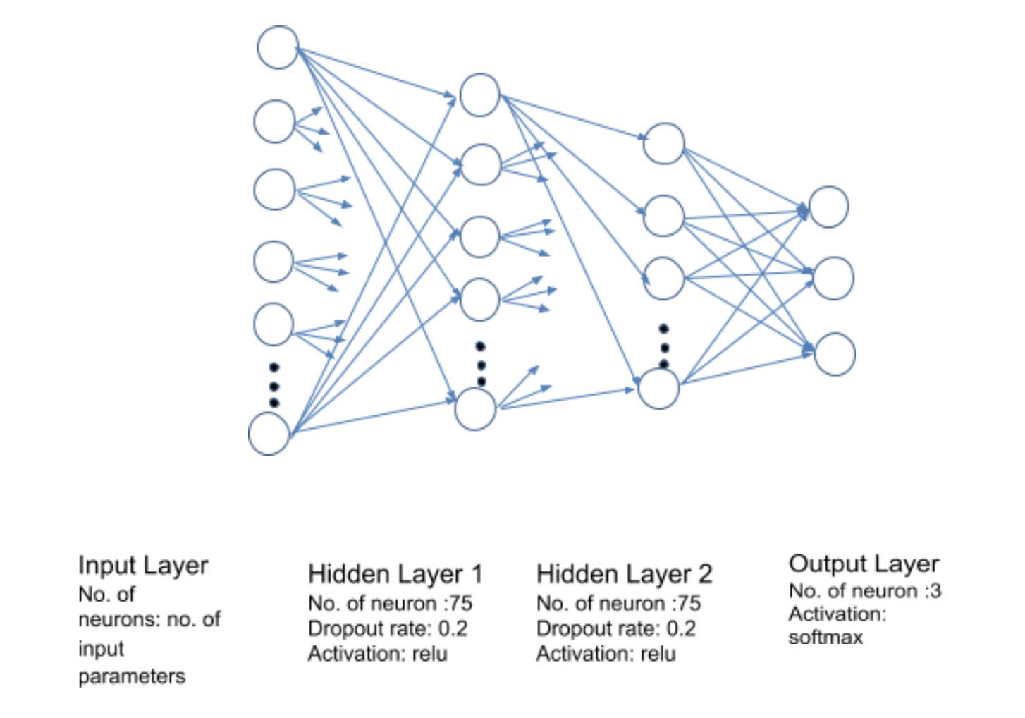
We have built many models to predict the outcome of 2018 world cup games: 1. Logistics Regression (LR), 2. Linear Discriminant Analysis (LDA), 3. k-Nearest Neighborhood (kNN), 4. Decision Tree (CART), 5. Gaussian NB (NB), 6. Support Vector Machines (SVM),  7.Random Forest (RF), 8. Gradient Boosting Classifier (GB), 9. AdaBoost Classifier (AB) and 10. Multilayer Perceptron (MLP) Neural Network. We pick a few of them to explain the process.

1. MLP Neural Network: A dense sequential layer neural network architecture is used.  We have come up with a network architecture with 2 hidden layers and 1 output layer. The number of neurons in the input layer is equal to the number of input parameters.  The number of neurons in hidden layer 1 is 100 and in hidden layer 2 is 75. The dropout rate 0.2 given at hidden layers to avoid overfitting.  The loss function to optimize at the output layer is categorical_crossentropy.  We have come up with the following parameters after trial and error.  

Optimizer = sgd with; learning rate = 0.9; decay rate = 0.02/num_epochs; batch_size = 512.

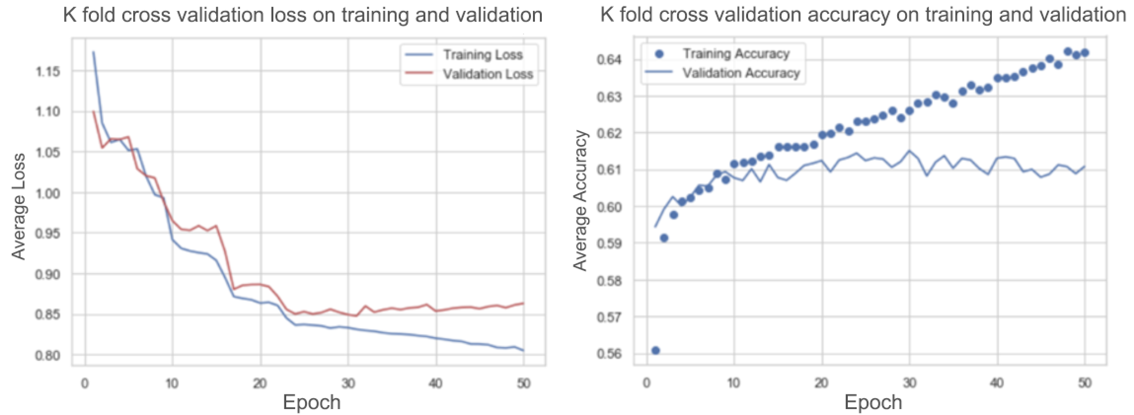
We experimented with different input data set generated using different missing value handling methods. The input data set where the missing values are imputed showed better performance than the input data with missing values removed one.  K – fold cross validation is done with 4 folds and 50 number of epochs to identify the optimal number of epochs for the network.  The cross validation mean accuracy and loss on training and valid data set shows that the model starts overfitting after 40 epochs.

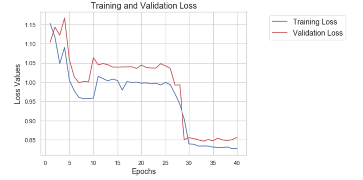
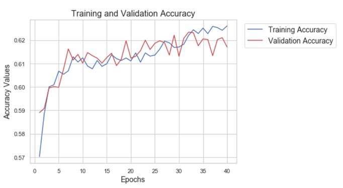
The model is re-trained using for 40 epochs, and the loss and accuracy score are monitored.  The trained model is used to predict the game outcome on test data set.  The model accuracy on validation set is 0.62 and on test data set is 0.51. This is somewhat of a disappointment and we guess it could be because the test set is quite different from the train set (like the example in HW9). The test set contains all the games played in Russia with many neutral games. We probably have to re-think how the training set needs to be considered. It is possible to take a smaller set where the test set is in good alignment with the train set (only World Cup matches?). However, given lack of time, we have not tried much in that direction and leave it for future work.

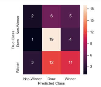
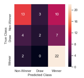
Confusion Matrix on Test data:

2. Support Vector Machine:

The support vector machine classifier is built with different kernels and regularization parameter.  The model with rbf kernel and regularization parameter C=1 produced better cross validation accuracy score of 0.61.  The trained model is used to predict the outcome of the 2018 world cup games (test data).  The accuracy score on the test data is 0.59.  

The confusion matrix shows that SVM classifier has high sensitivity to Winner class.

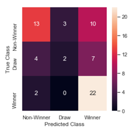
3.         Ada Boosting Classifier:

The ada-boosting classifier is built and trained on the training data. We experimented with different parameter settings for number of estimator, learning rate and found that the default setting of  n_estimators = 50  and learning rate learning_rate =1 and SAMME.R ada-boosting algorithm produced better cross validation accuracy of 0.61.  The trained ada boost model is used to predict the outcome on the test data.  The accuracy score on the test data is 0.59.

The confusion matrix for test data shows that Ada boosting classifier has high sensitivity to Winner class.

Comparison of Model Performance

Comparing all the above four models shows that neural network does not give better accuracy score on test data though it has higher accuracy score on cross validation set.  SVM and Ada Boosting give same accuracy score on cross validation and test data.  It shows that neural network overfitted to training data though we have introduced drop outs and regularization parameters.  In terms of running time, the SVM is very slow and computationally very expensive.  Ada boosting is built on week learners, and it converges very quickly.  

Comparative Study on Different Classifiers

We wanted to experiment with the different classifiers to understand how different classifiers perform on world cup data.

Models considered in the analysis:

1.     Logistic Regression – liblinear solver

2.     Linear Discriminant Analysis

3.     K-Nearest Neighborhood Classifier

4.     Decision Tree Classifier - loss function gini score

5.     Naïve Bayes Classifier

6.     Support Vector Machine Classifier - loss function squared_hinge

7.     Random Forest Classifier – loss function gini score

8.     Gradient Boosting Classifier -  loss function MSE

9.     Ada Boost Classifier

We used the default parameter setup in sklearn for all the models in order to have the fair comparison of the models.

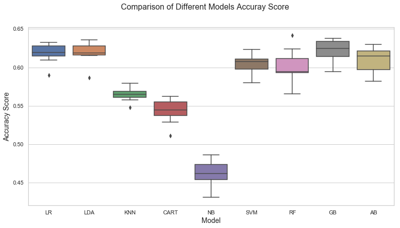
Ten-fold cross validation is used to measure the consistency of the performance metrics.  The accuracy score is used as a measure of performance.  The box plots show the median accuracy score and the spread of the accuracy scores.  The top winning models are logistic regression, linear discriminant analysis, gradient boosting classifier and Ada boost classifier.  The top performance models have mean accuracy score around .63.  The SVM and Random Forest models are closer to top performing models.   The Naïve Bayes classifier is the worst model which has the median accuracy score around .46 which is very low compared to top performing models.  The results of the decision tree is a surprise to us, the accuracy score of decision tree is lower than the KNN model.  It shows that the decision tree might have difficulty to find a best split with too many categories in team 1 and team 2 feature and have overfitting issue.  Boosting models (Gradient Boosting and Ada Boosting) are robust to overfitting and shows good performance score.

Performance Metrics Comparison

The performance of all 9 models are tested on the test data set.  The test data set accuracy shows that the ada boosting has top accuracy score of 0.62

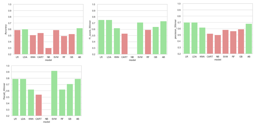
Models Performance on predicting the Winner class:

The accuracy plot on winner class shows that the Ada boosting and Linear Discriminant Analysis performs well on predicting the winner class.  The overall metrics f1-score shows that the overall performance of Decision Tree and Naïve Bayes models are low on predicting the winner class. The high recall score of the SVM shows high sensitivity on predicting the winner class.

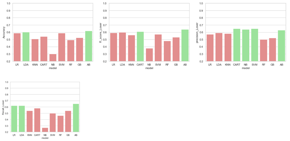
Models Performance on predicting the Loser class:

The accuracy plot on loser class shows that the Ada boosting and Linear Discriminant Analysis performs well on predicting the loser class.  The overall metrics f1-score shows that Decision Tree and Ada boosting have high performance on predicting the loser class. The high recall score of the Ada boosting shows high sensitivity on predicting the loser class.

Based on our comparative analysis, we conclude that Boosting Models: Ada boosting, Gradient Boosting,  SVM, Logistic regression and Random Forest Models can be used to model the world cup game prediction problem.

Fine-tuning of Random Forest Model (Best Model)

From the charts, we can see several models hitting about 60-65% accuracy. Given more time, we could try tuning the models further. However, when the  Random Forest model was tuned, we were able to achieve a score of 66.67% on the test set (when including draws), which seems to be our best score achieved. This was achieved by limiting the number of trees to 500 and stopping at a maximum depth of 9. If we spend more time on the other models and tune them further, they might achieve this accuracy or even better but for the sake of this project our best model is Random Forest with 66.67% accuracy on the test set.

Accuracy of Final Random Forest model on train set:  67.52 %

Accuracy of Final Random Forest model on test set:  66.67 %